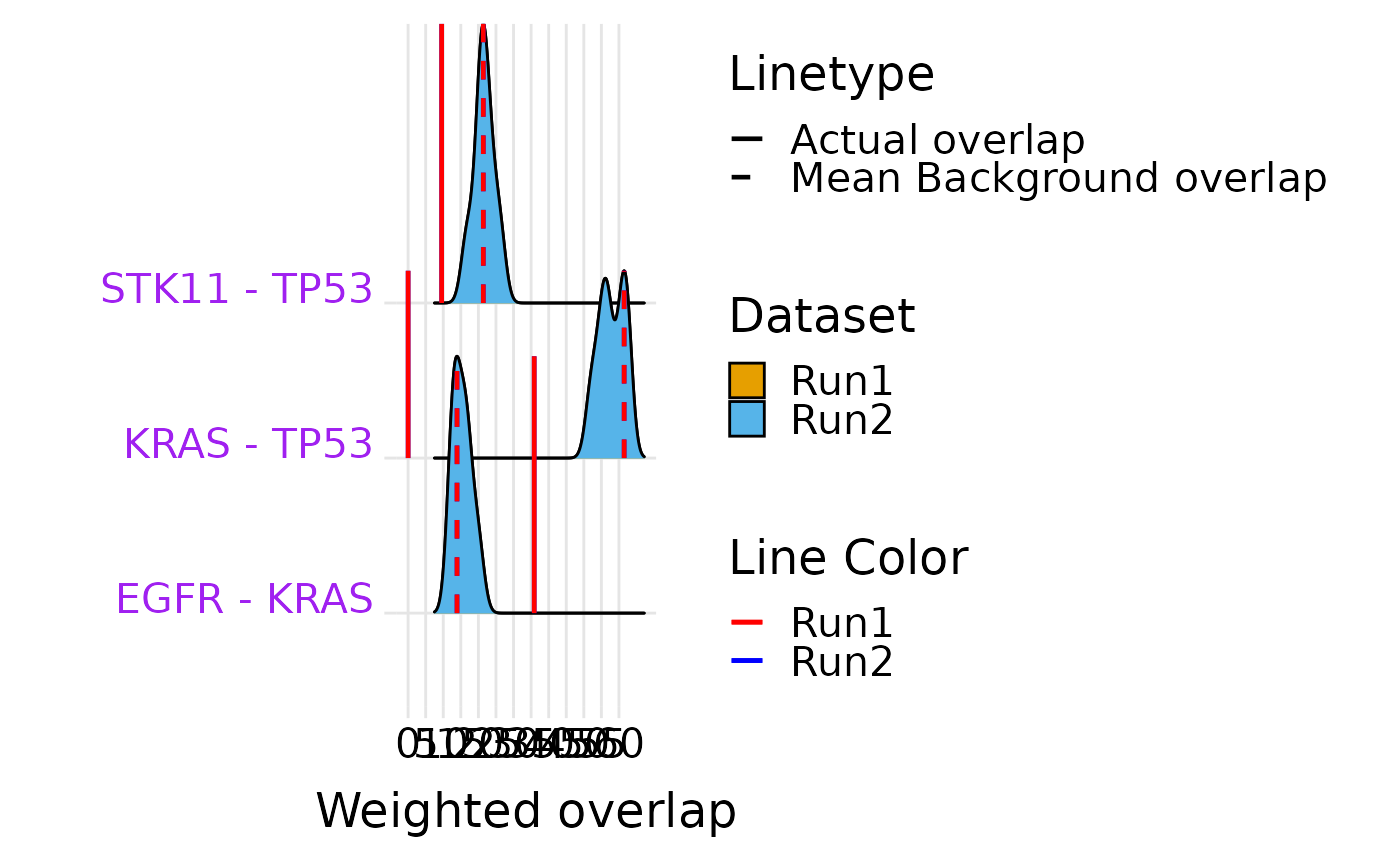
Ridge plot comparing null-model distributions for two datasets
Source:R/selectX_plot.R
ridge_plot_ed_compare.RdFor each gene pair in result_df, overlays the null-model weighted-overlap
distributions from two separate selectX runs, allowing visual comparison
of evolutionary dependencies across cohorts or conditions.
Arguments
- result_df
A data frame of gene pairs to display, with columns
SFE_1,SFE_2,name,type,dataset1_w_overlap, anddataset2_w_overlap.- obj1
SelectX object for dataset 1 (
selectX()$obj).- obj2
SelectX object for dataset 2 (
selectX()$obj).- name1
Display label for dataset 1.
- name2
Display label for dataset 2.
Examples
# \donttest{
data(luad_run_data, package = "SelectSim")
r1 <- selectX(M = luad_run_data$M,
              sample.class = luad_run_data$sample.class,
              alteration.class = luad_run_data$alteration.class,
              n.cores = 1, min.freq = 10, n.permut = 10, verbose = FALSE)
r2 <- selectX(M = luad_run_data$M,
              sample.class = luad_run_data$sample.class,
              alteration.class = luad_run_data$alteration.class,
              n.cores = 1, min.freq = 10, n.permut = 10, verbose = FALSE)
common <- head(r1$result, 3)
common$dataset1_w_overlap <- common$w_overlap
common$dataset2_w_overlap <- common$w_overlap
ridge_plot_ed_compare(common, r1$obj, r2$obj, "Run1", "Run2")
#> Picking joint bandwidth of 1.68
#> Warning: Arguments in `...` must be used.
#> ✖ Problematic argument:
#> • alpha = 0.2
#> ℹ Did you misspell an argument name?
#> Warning: Vectorized input to `element_text()` is not officially supported.
#> ℹ Results may be unexpected or may change in future versions of ggplot2.
#> Picking joint bandwidth of 1.68

# }
# }